What is Artificial Intelligence?

Lesson 1

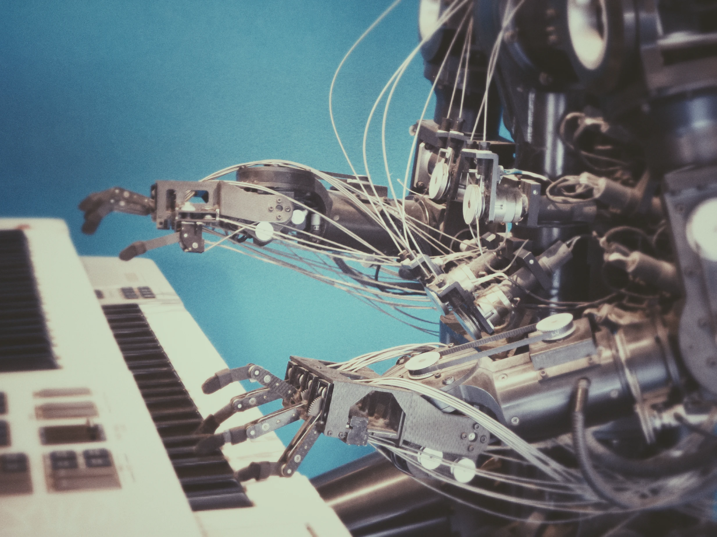
Movies and book have depicted a generalized AI, one that can answer any question we might have, and do anything a human can do. Unfortunately, this is not realistic.

A machine is said to have artificial intelligence if it can interpret data, potentially learn from the data, and use that knowledge to adapt and achieve specific goals.

Some more obvious uses of AI include Alexa, Roomba, Siri, and more. But, there are a ton of less obvious examples! When we buy something in a big store or online, AI decides which and how many items to stock. When we scroll through Facebook or Instagram, AI decides which ads we see.

AI even affects big life decisions. For example, when you submit your college or application, AI might be screening it before a human even sees it.

AI and automation is changing everything, from commerce to jobs. This change is global, some people are excited about it, and others are afraid of it. Either way, we all have the responsibility to understand AI and figure out what role AI will play in our lives.

Close Lesson

Supervised Learning

Lesson 2

Humans are not born with many skills. We need to learn how to sort mail, land airplanes, and have friendly conversations. Computer scientists have tried to teach computers how to learn like we do, with a process called supervised learning.

The process of learning is how anything can make decisions. Humans, animals, or AI systems can adapt their behavior based on their experiences.

We will discuss three types of learning:
1. Reinforcement learning is the process of learning in an environment through feedback from an AI's behavior. Think about how babies learn to walk. Nobody teaches a baby how to walk, but they learn from their experiences of practicing and stumbling, until they can put one foot in front of the other.
2. Unsupervised learning is the process of learning *without* training labels. It is also known as clustering or grouping. Sites like Youtube use unsupervised learning to find patterns and frames of videos, and compress those frames so videos can be streamed to us quickly.
3. Supervised learning is the process of learning *with* training labels. It is the most widely used kind of learning when it comes to AI. We will discuss supervised learning in more detail below.

To explain supervised learning, we will walk through a few examples.

Regression

Suppose we have a dataset containing house sizes and prices in Portland, Oregon. Our goal is to predict housing prices.

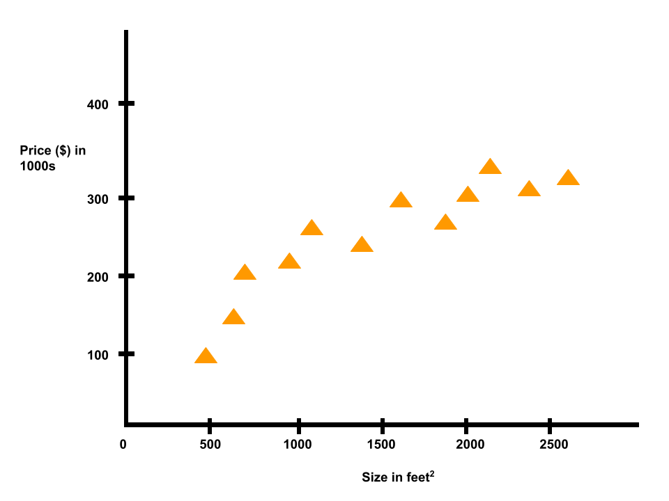
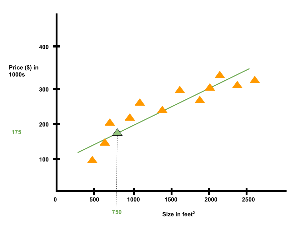
Given the data, let's say we have a friend who owns a house that is 750 sq feet and our friend wants to know how much to sell the house for. One learning algorithm would be to put straight line through data and based on that, maybe sell the house for 175k.

Instead of fitting a straight line, we could also fit a quadratic function to the data and based on that, maybe sell the house for 240k.

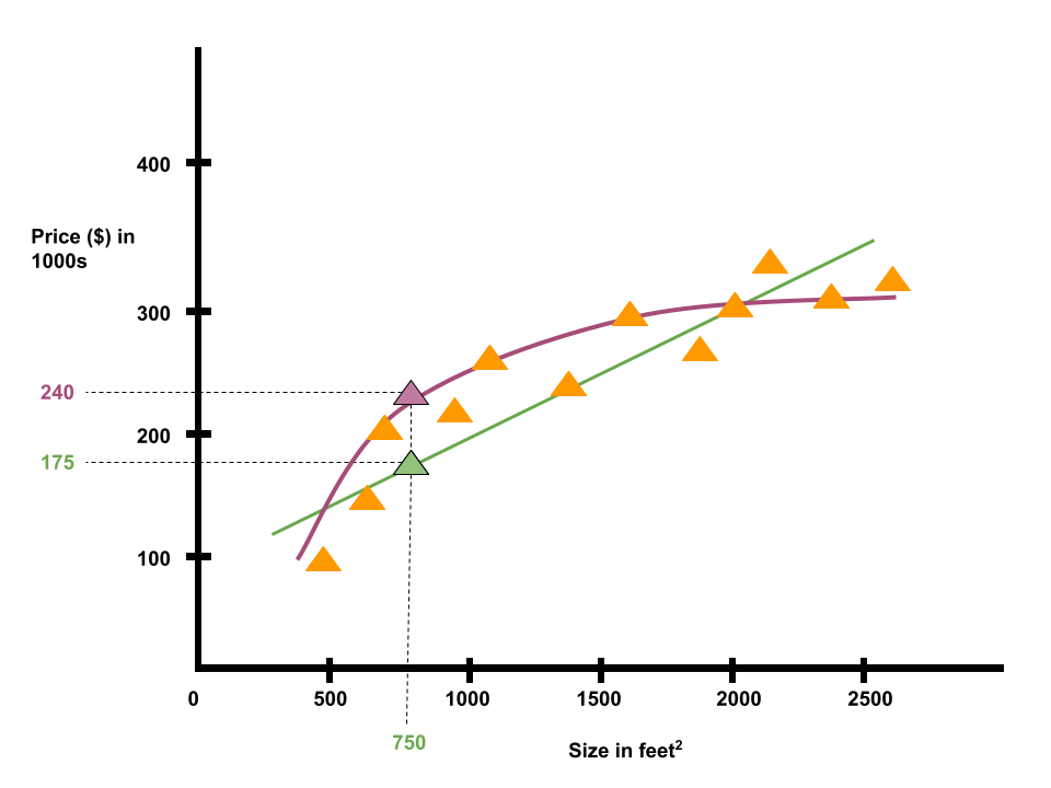
This is an example of a supervised learning algorithm. Supervised learning refers to the fact that we provide the algorithm with a dataset where the "right answers" are given.

In the housing problem, for every example in the dataset, we provided the right price that the house sold for. Our task was to produce more of these right answers. This is called a regression problem, where we predict continous valued outputs (which, in this case, is price of the house).

Next, we will look at another supervised learning example.

Classification

Suppose we have a bunch of donuts and bagels, and we want to be able to determine whether or not some food is a donut. Suppose we have 5 examples of donuts and 5 examples of bagels, and we know the mass of each food item in grams.

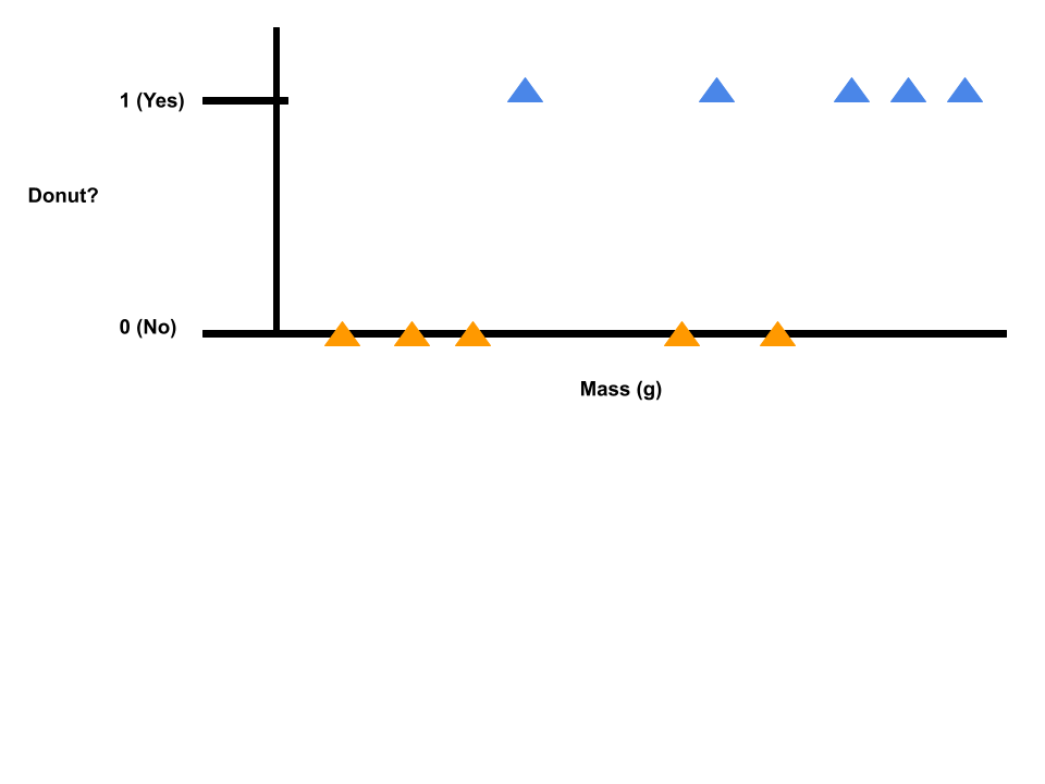
Let's say we have a food item. We want to estimate the probability that the food item is a donut.

This is an example of a classification problem, where we have discrete valued outputs (0 or 1). Note that it is possible to have more than two possible values for the output (e.g., if we wanted to classify food as donut, bagel, or croissant).

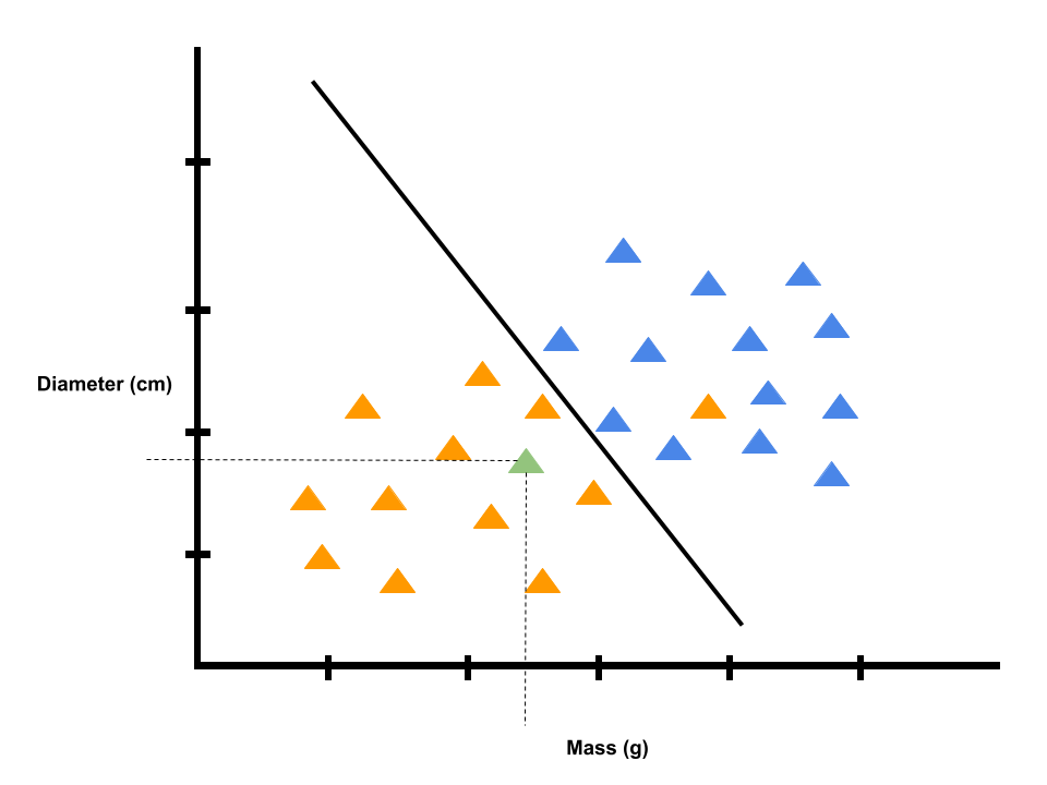
We can also draw our donut and bagel data as follows. Note that we take the original plot of the dataset and map it down to a real line. The orange triangles indicate bagel examples (non-donut examples) and the blue triangles indicate donut examples.

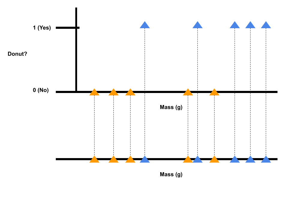
In this example, we use only one feature or attribute (i.e., mass in grams). Suppose we know the diameter of the food items in centimeters in addition to the mass in grams.

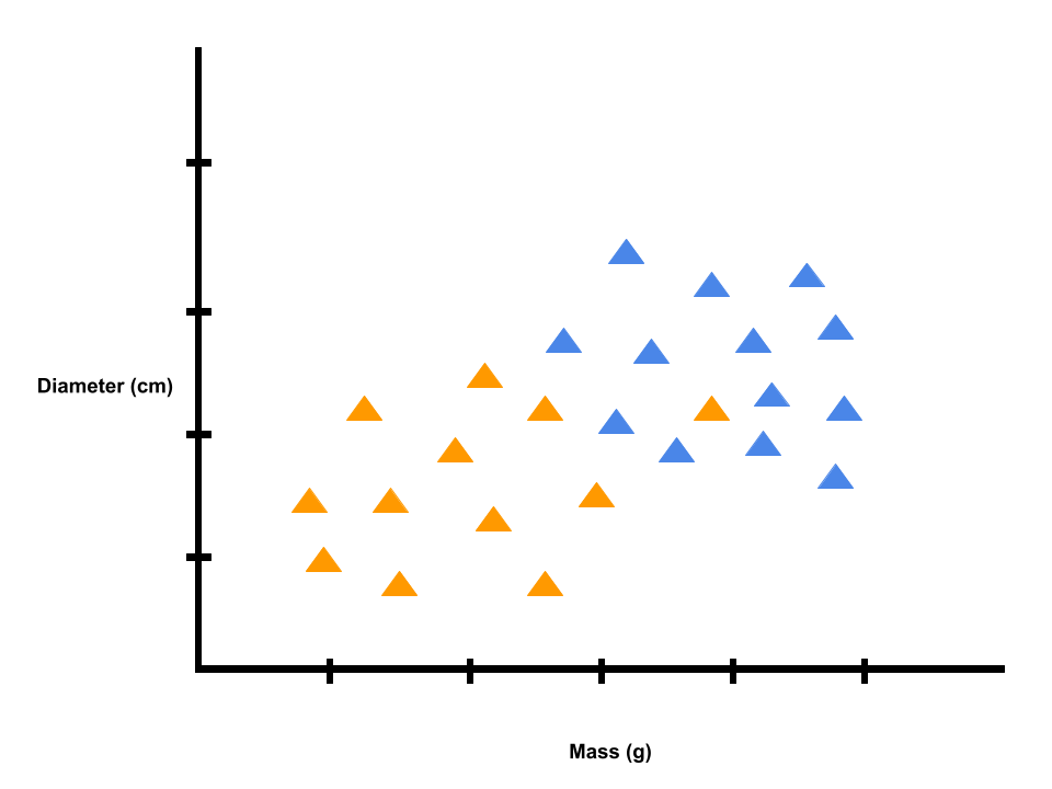
Let's say we have a food item, as indicated by the green triangle. We want to estimate the probability that the food item is a donut. The learning algorithm can draw a straight line through the data to try to separate the donuts from bagels.

Based on where the green triangle falls with respect to the decision boundary, we would decide it is more likely that the food item is a bagel than it might be a donut. So, we would classify the food item as a bagel.

In this example, we had two features: mass and diameter. In other machine learning problems, we might have more features.

Exercise

Based on what we've learned, let's do a quick exercise.

You are running a company and you want to develop learning algorithms to address each of the two problems.
Problem 1: You have a large inventory of identical items. You want to predict how many of those items will sell over the next three months.
Problem 2: You'd like software to examine individual customer accounts, and for each account decide whether it has been hacked/compromised.

Should you treat these as classification or regression problems?
A) Treat both problems as classification problems
B) Treat problem 1 as a classification problem and problem 2 as a regression problem
C) Treat problem 1 as a regression problem and problem 2 as a classification problem
D) Treat both problems as regression problems

The correct answer is C.

Sources

1. Lecture 1.2 — Supervised Learning — Machine Learning by Andrew Ng
2. Supervised Learning: Crash Course AI #2

Close Lesson

The Perceptron

Lesson 3

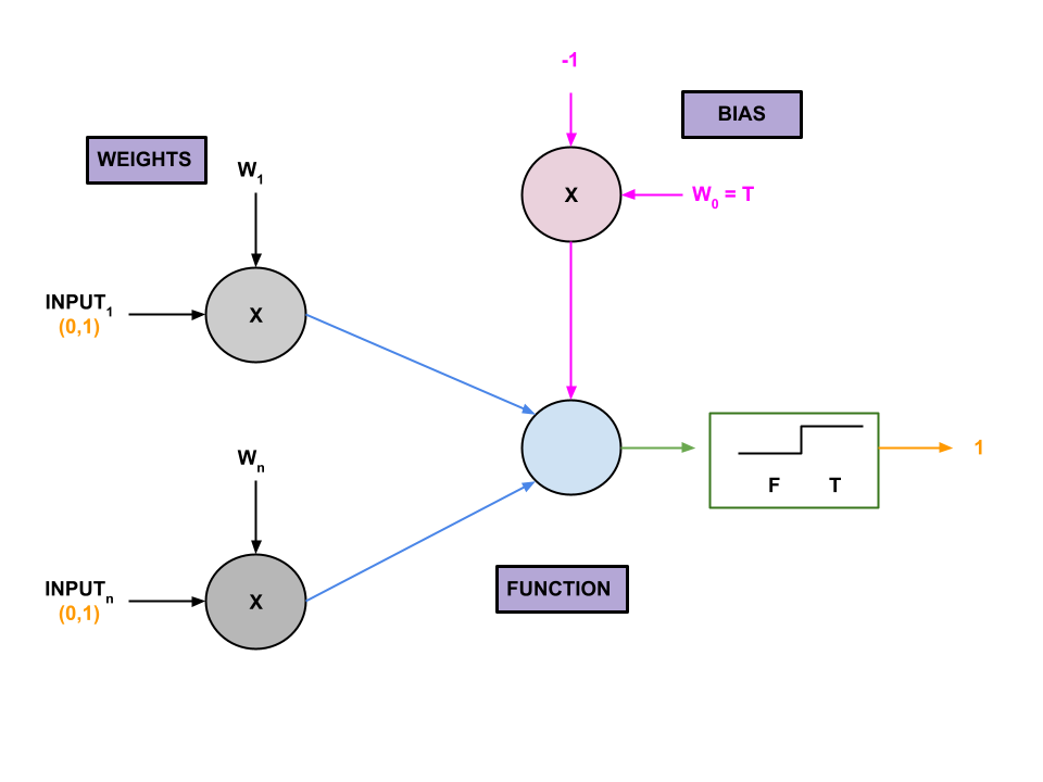
In 1958, a psychologist named Frank Rosenblatt was inspired by the Darmouth conference to create an artificial neuron. His goal was to teach this AI to classify images as triangles or not triangles using his supervision (hence, supervised learning). He called this machine the perceptron.

He attached the perceptron to a camera. He would show the camera a picture of a triangle and not triangle (e.g. a circle). Depending on whether the camera saw ink or paper in each spot, each pixel would send a different electric signal to the perceptron. Then, the perceptron would add up all the signals that matched the triangle shape.

If the total charge was above its threshold, it would send a send an electric signal to turn on a light.
>> Yes, that's a triangle!

But, if the electric charge was too weak to hit the threshold, the machine would not do anything, and the light would not turn on.
>> No, that's not a triangle!

At first, the perceptron was basically making random guesses. To train the perceptron with supervision, Rosenblatt used yes and no buttons.

If the perceptron was correct, he would push the yes-button, and nothing would change.

If the perceptron was wrong, he would push the no-button, which would set off a chain of events that adjusted how much electricity crossed the synapses and adjusted the machine's threshold level. This made the perceptron more likely to get the answer correct next time.

Nowadays, we can use modern computers to program AI to behave like neurons.
First the artificial neurons receives inputs multiplied by different weights, which correspond to the strength of each signal.

The threshold is represented by a special weight called the bias, which can be adjusted to raise or lower the neuron's eagerness to fire.

All the inputs are multiplied by their respective weights, added together, and a mathematical function gets the result.

In the simplest AI systems, this function is called a step function, which can only output a 0 or 1.

If the sum is less than the bias, then the neuron will output a 0, which could indicate not-triangle (or, something different depending on the task).

If the sum is greater than or equal to the bias, then the neuron will output a 1, which indicates the opposite result.

An AI can be trained to make a decision about anything, where you have enough data and supervised labels.

Bagels vs. Donuts Example

Bagels and donuts might look super similar to each other, so we want to be able to distinguish between the two.

Suppose we measure the mass and diameter of bagels, and supervise a program so it gets better at labeling them. Initially, the program does not know anything about bagels, donuts, or what their masses or diameters might be. The program will initially use random weights for mass, diameter, and bias to make a decision between whether something is a donut or bagel. As the program learns, the weights will be updated.

We can use different mathematical functions to account for how far an AI is from the right decision.

We'll keep it simple and use a step function (an either-or-choice, like bagel or donut).

Let consider a mixed bag of donuts and bagels. Suppose we pull out our first item, and it happens to be a donut with a mass of 34 grams and a diameter of 7.8 cm. The perceptron takes these inputs, multiplies them by their respective weights, and adds them together.

The bias is like the bagel threshold. If the summer is greater than or equal to the bias (which is the threshold for the neuron firing), the program will output bagel. If the sum is less than the bias (i.e. it has not crossed the bagel threshold), the program will output donut.

We can think of this program as a graph, with the mass on one axis and the diameter on the other. The weights and bias are used to calculate a line called a decision boundary on the graph, which separates bagels from donuts.

If we represent this bagel as a data point, we would graph it at (20, 5). This data point is above the decision boundary, and therefore in the bagel zone. Thus, when we ask the program what the first item we pulled out of the bag is, the program will output bagel, which is wrong because the item is a donut.

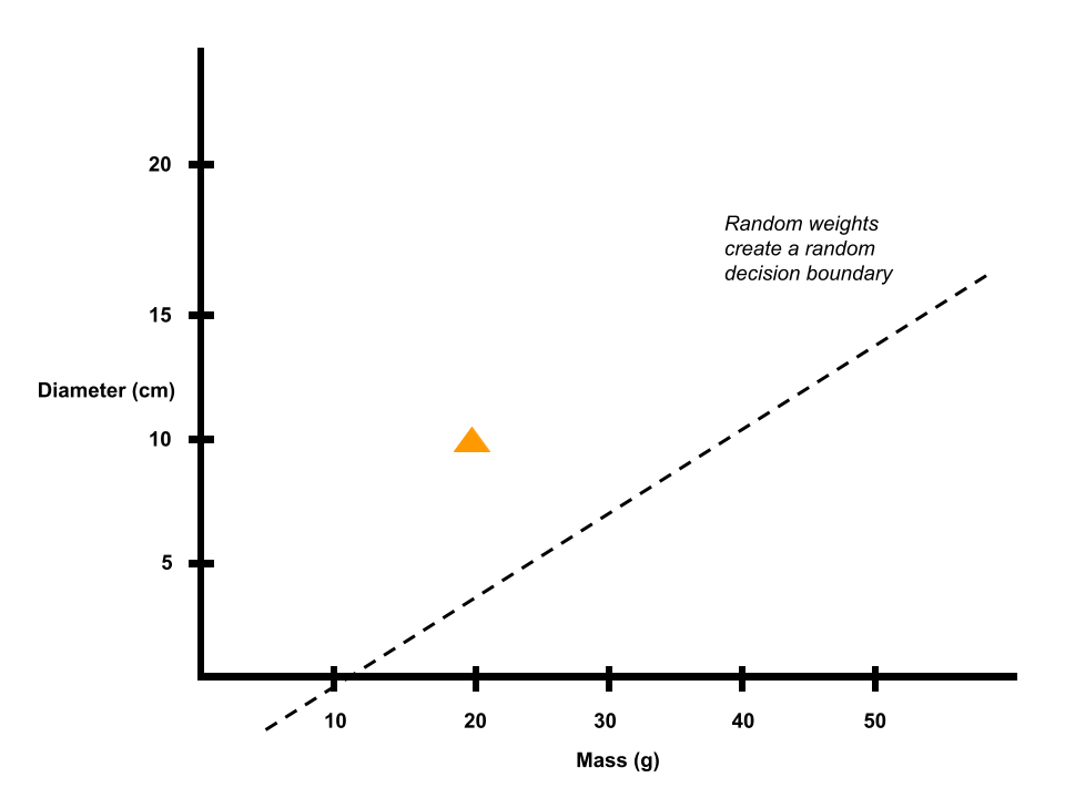
Since the program is initially using random weights, the program essentially makes a random guess. We can help the program learn by updating its weights. So, we take an old weight and add a number calculated with an equation called an update rule.

Because our perceptron can be completely right or completely wrong, the update rule is relatively simple.

If the program makes the right prediction of labelling the donut as a donut, we add 0 to the weight, and the weight stays the same.

But, if the program makes the wrong prediction and labels the donut as a bagel, the update rule has a value, which is a small positive or small negative number. We will add that value to the weight, and the weight will change.

Conceptually, this means the program learns from failure, but not from success.

We pulled a donut out of the bag, and the program predicted that the item was a bagel. So, we will let the program know that it made the wrong choice, and it will consequently update its weights.

When the weights update, the decision boundary changes. The datapoint we added is now below the decision boundary line and in the donut zone.

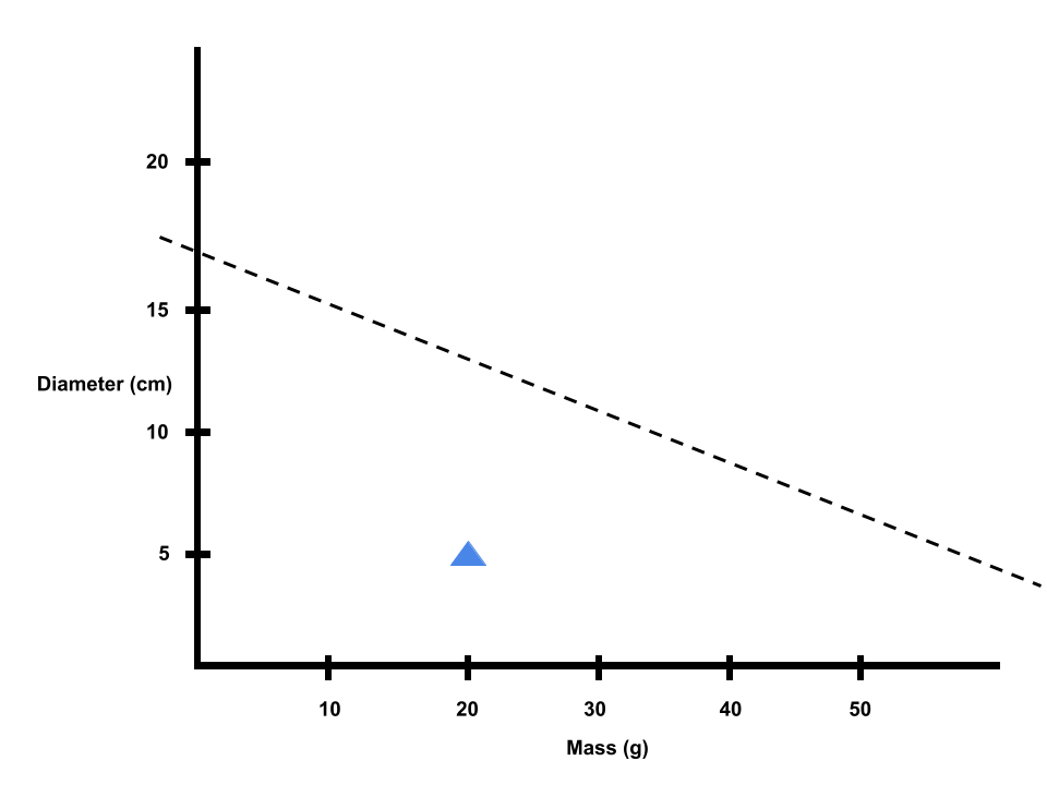
Now, the program will classify another item with this mass and diameter as a donut.

Suppose we pull out a second item with a mass of 40 grams and a diameter of 2.5 cm. We give this to the program, and it predicts that the item is a donut correctly. The data point appeared below the decision boundary in the donut zone.

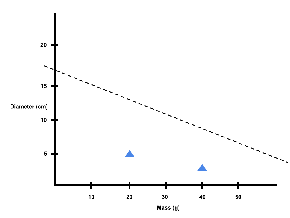
We let the program know that its prediction was correct, so the weights stay the same and so does the decision boundary.

Now, we can do this many more times to train the program's perceptron.

After we have trained the program, we have to test it on a bunch of new data to see how well the program learned. We can visualize the results in a confusion matrix. We can add together what the program got right and dividing by the total number of items to get the test accuracy.

	Predicted Donut		Predicted Bagel	Total
Actually Donut	8		17	25
Actually Bagel	2		73	75
Total	10		90	100 Total

Test Accuracy = (8 + 73)/ 100 = 81%

To really understand what is wrong, we can look at the precision and recall.

Precision tells you how much you should trust your program when it says it found something. Of the 10 donuts we gave the program, it said 8 of them were actually donuts, so the program is 80% precise, and we can be 80% sure that the program is giving us donuts when the items are actually donuts.

Recall tells you how much your program can find the thing you are looking for. Of the 25 items that were donuts, the program correctly labelled 8 of them. So, the program's recall is 32%.

The precision and recall depend on the criteria the program is using to make a decision. As we can see in the graph below, the program generally thinks that donuts generally have smaller diameter and mass than bagels.

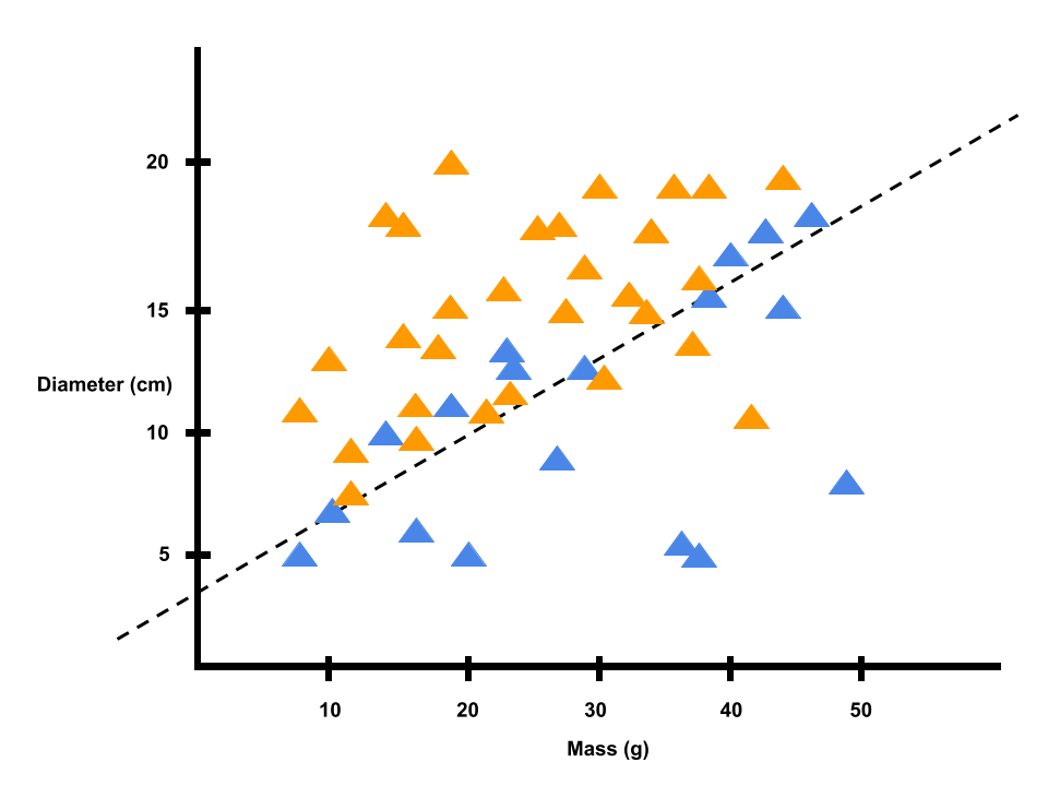
When it comes to classifying donuts, the program has high precision because if it says something is a donut, we're pretty sure it is actually a donut. But the program has some recall, because some donuts can be bigger than the donuts we used to train the perceptron program and might fall in the bagel zone.

Figuring out what criteria to use is the key for most AI challenges. If we wanted better accuracy for this donut vs. bagel problem, we could have used inputs other than mass and diameter, such as checking for whether the item has seeds or sprinkles.

Sources

1. Supervised Learning: Crash Course AI #2

Close Lesson

Neural Networks (Pt. 1)

Lesson 4

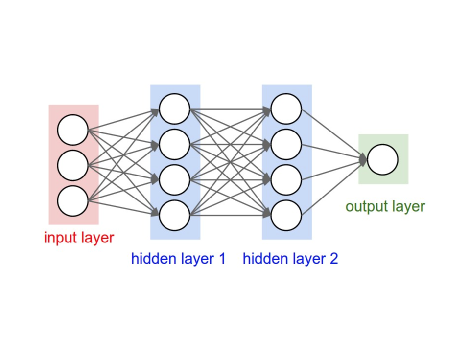
Previously, we looked at a perceptron (a program that imitates one neuron). But, our brains make decisions based on hundreds of millions of neurons, which have trillions of connections between them.

We can do a lot more with AI if we connect a bunch of perceptrons together to create what is called an artificial neural network.

Neural networks are better for tasks like image recognition. The secret to their success is hidden layers. All neural networks are made up of an input layer, an output layer, and any number of hidden layers in between.

There are many different arrangements, but we will look at the classic multilayer perceptron. The input layer is where the neural network receives input data represented as numbers. Each input neuron represents a single feature,which is some characteristic of the data. Features are straightforward if we are talking about something that’s already a number, (e.g. grams of sugar in a donut). But, just about anything can be represented as a number. Sounds can be represented as the amplitudes of the sound wave (so, each feature would have a number representing the amplitude at a moment in time). Words in a paragraph can be represented by how many times each word appears (so, each feature would be the frequency of one word).

If we are trying to label an image of a dog, each feature would represent information about a pixel. For a grayscale image, each feature would have a number representing how bright a pixel is, but for a colored image, we can represent each pixel with 3 numbers (the amount of red, green, and blue).

Once the features have data, each one sends its number to every neuron in the next layer (which is called the hidden layer). Then, each hidden layer neuron mathematically combines all the numbers it gets.

The goal is to measure whether the input data has certain components.

In an image recognition problem, these components can be a color in the center, a curve near the top, or even whether the image contains eyes, ears, or fur.

Instead of answering yes or no like in the perceptron, each neuron in the hidden layer does some complicated math and outputs a number. Then, each neuron sends its number to every number in the next layer, which could be another hidden layer or the output layer. The output layer is where the final hidden layer outputs are mathematically combined to answer the problem. Let’s say we are trying to label an image as a dog. We might have a single output representing a single answer (that the image is a dog). But, if there are many answers, we’ll need a bunch of output neurons. Each output neuron corresponds to the probability for each label (e.g. dog, cat, bird, and more). We pick the answer with the highest probability.

Sources

1. Neural Networks and Deep Learning: Crash Course AI #3
2. TensorFlow NN+Drop out+Batch Norm(LB 0.515)

Close Lesson

Neural Networks (Pt. 2)

Lesson 5

Neural networks handle mistakes using an algorithm called backpropagation to make sure all the neurons that contributed to an error get their math adjusted.

Neural networks have two main parts:
1. The architecture
2. The weights

The architecture includes neurons and their connections. The weights are numbers that fine-tune how the neurons do their math to get an output. If a neural network makes a mistake, usually, the weights aren’t adjusted correctly and we need to update them so they make better predictions next time. The task of finding the best weights for a neural network architecture is called optimization.

To better understand optimization, let’s start with an example.

Suppose we have a dataset containing house sizes and prices in Portland, Oregon. Our goal is to predict housing prices. A simple way to do this is by graphing those data points.. Then, we can look for a pattern in that graph to make predictions. A way computers do this is with an optimization strategy called linear regression. We start by drawing a random straight line on the graph, which kind of fits the data points.

To optimize, we need to know how incorrect this guess is. Hence, we calculate the distance between the line and each of the data points, add it all up, and that gives us the error (note that we are quantifying how big of a mistake we made).

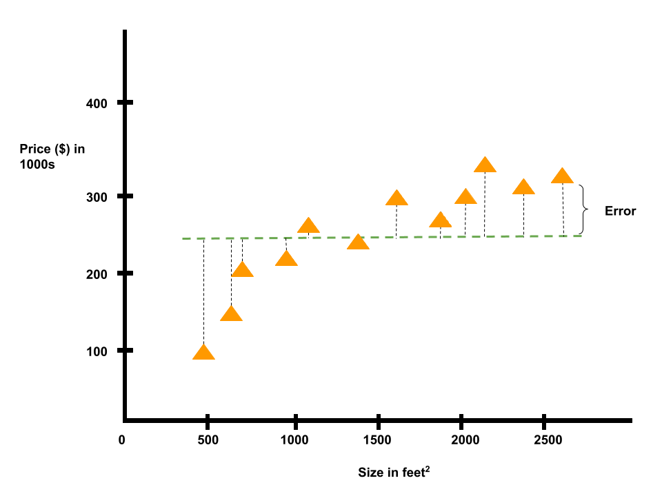
The goal of linear regression is to adjust the line to make the error as small as possible. We want the line to fit the training data as much as it can. The result is called the line of best fit. We can use this straight line to predict the price of a house in Portland, Oregon.

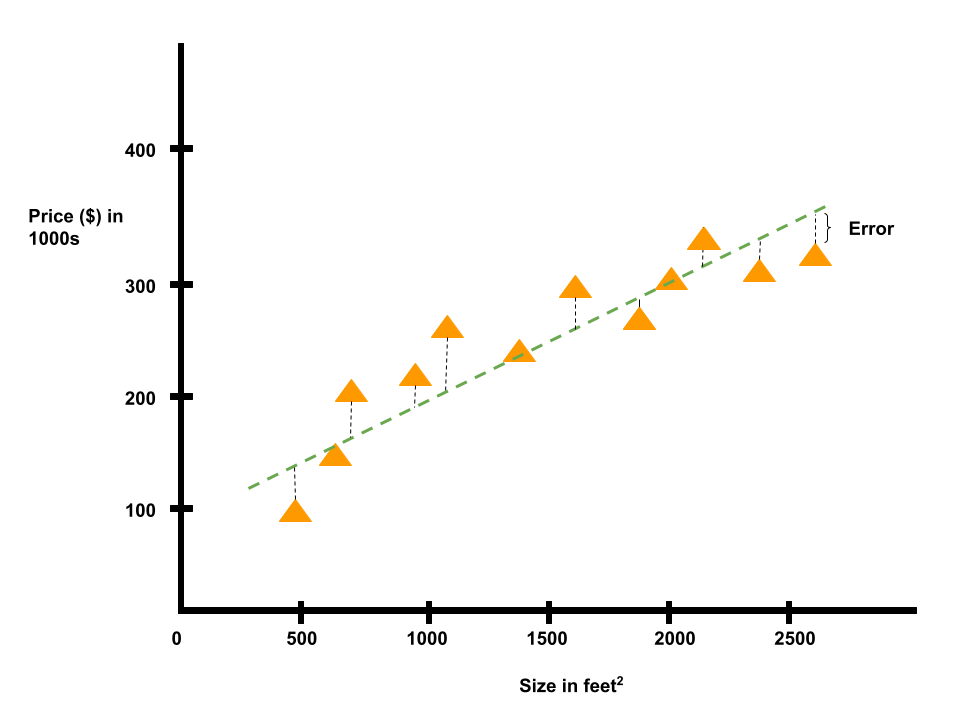
To get more accurate results, we might want to consider more than two features, like for example adding the number of bathrooms in the residence, which would turn our 2d graph into 3d. And our line of best fit would be more like a plane of best fit. But if we added a fourth feature, like the number of floors in the residence, we can’t visualize this anymore. As we consider more features, we add more dimensions to the graph, the optimization problem gets trickier, and fitting the training data is tougher.

This is where neural networks come in handy.

By connecting together many simple neurons with weights, a neural network can learn to solve complicated problems, where the line of best fit becomes a weird multi-dimensional function.

### Training Neural Networks To stick with the same example, the input layer of this neural network takes features like square footage of the house, the number of bathrooms, number of floors, and so on. The output layer predicts the price of the house.

Let’s ignore the architecture of the neural network for now and focus on the weights. We begin by setting the weights to random numbers, like the random line on the graph we drew earlier. Note that this time, it’s not just one random line because we have lots of inputs, so it is a lot of lines that are combined together to make one function.

To train this neural network, we will give the network access to the dataset because we also know the price of each house in the dataset. The neurons will multiply those features by the weights, add the results together, and pass information to the hidden layers until the output neuron has an answer.

Suppose for the house of 500 sq feet, the neural network outputs the price $145k, and the true price is $100k. There is a difference between the neural network’s output and the actual price of each house. Because we just have one output neuron, that difference of 45k is the error.

In some neural networks though, the output layer may have a lot of neurons, so the difference between the predicted answer and the correct answer is more than just one number.

In these cases, the error is represented by what’s known as a loss function. Moving forward, we need to adjust the neural network’s weights so that the next time we give the neural network similar inputs, its math and final output will be more accurate. We need the neural network to learn from its mistakes, which is similar to the supervisor button idea when we were discussing the perceptron program. a button to supervise his learning when he had the perceptron program.

Backpropagation helps neurons learn. The basic goal is to look at the loss function and then assign blame to neurons back in the previous layers of the network. Some neurons’ calculations may have been more to blame for the error than others, so their weights will be adjusted more.

This information is fed backwards, which is where the idea of backpropagation comes from. For example, the error from our output neuron would go back a layer and adjust the weights that get applied to our hidden layer neuron outputs. The error from our hidden layer neurons would go back a layer and adjust the weights that get applied to our features.

A Metaphor for Backpropogation

Recall that our goal is to find the best combination of weights to get the lowest error. To explain the logic behind optimization with a metaphor, let’s imagine that weights in our neural network are like latitude and longitude coordinates on a map. The error of our neural network is the altitude -- lower is better. The neural network is where the explorer is on a quest to find the lowest point in the deepest valley. The latitude and longitude of that lowest point -- where the error is the smallest -- are the weights of the neural network’s global optimal solution.

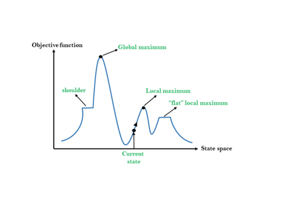
The neural network has no idea where this valley actually is. By randomly setting the initial weights of our neural network, we’re basically dumping our model in the middle of nowhere. All the model knows is its current latitude, longitude, and altitude.

We might be lucky and be on the side of the deepest valley. However, we could also be at the top of the highest mountain somewhere far away. The only way to know is to explore by looking around and making a guess.

Suppose we notice that we can descend down a little by moving northeast, so our model takes a step down and updates its latitude and longitude. From this new position, the model looks around and picks another step that decreases its altitude a little more. With every step, the model updates its coordinates and decreases its latitude.

Eventually, the model looks around and finds that it cannot go down anymore. Thus, the model thinks it has found the lowest point in the deepest valley. However, if we look at the whole map, we can see that our model found the bottom of a small gorge when it ran out of “down.” This solution is better than where the model started, but is not the lowest point of the deepest valley. This is called a local optimal solution, where the weights make the error relatively small, but not the smallest it could be.

Backpropagation and learning always involves lots of little steps, and optimization is tricky with any neural network. Referring to our previous example of optimization as exploring a metaphorical map, we’re never quite sure if we’re headed in the right direction or if we’ve reached the lowest valley with the smallest error -- again that’s the global optimal solution.

But, we can use some tricks to help us better navigate. For example, when we drop an explorer somewhere on the map, they could be really far from the lowest valley, with a giant mountain range in the way. It might be a good idea to try different random starting points to be sure that the neural network isn’t getting stuck at a locally optimal solution.

Or instead of restarting over and over again, we could have a team of explorers that start from different locations and explore the jungle simultaneously.

We could even adjust the explorer’s step size, so that they can step right over small hills as they try to find and descend into a valley. This step size is called the learning rate, and it’s how much the neuron weights get adjusted every time backpropagation happens.

Ultimately, we’re looking for ways to minimize the loss function as we train neural networks. But even if we use a bunch of training data and backpropagation to find the global optimal, we still need to make sure that the system can answer new questions.

It’s easy to solve a problem we’ve seen before, like taking a test after studying the answer key. We may get an A, but we didn’t actually learn much. To really test what we’ve learned, we need to solve problems we haven’t seen before. The same is true for neural networks.

More data can be better for finding patterns and accuracy, as long as the computer can handle it. Over time, backpropagation will adjust the neuron weights, so that the neural network’s output matches the training data.This is called fitting to the training data, and with this complicated neural network, we’re looking for a multi-dimensional function.

Sometimes, backpropagation is too good at making a neural network fit to certain data. There are lots of coincidental relationships in big datasets. For example, the divorce rate in Maine may be correlated with U.S. margarine consumption, or skiing revenue may be correlated with the number of people dying by getting trapped in their bedsheets. Neural networks are really good at finding these kinds of relationships. This can be a big problem, because if we give a neural network some new data that doesn’t adhere to these silly correlations, then it will probably make some strange errors. That’s a danger known as overfitting.

Sources

1. Training Neural Networks: Crash Course AI #4
2. TensorFlow NN+Drop out+Batch Norm(LB 0.515)
3. Understanding Hill Climbing Algorithm in Artificial Intelligence

Close Lesson

Unsupervised Learning

Lesson 6

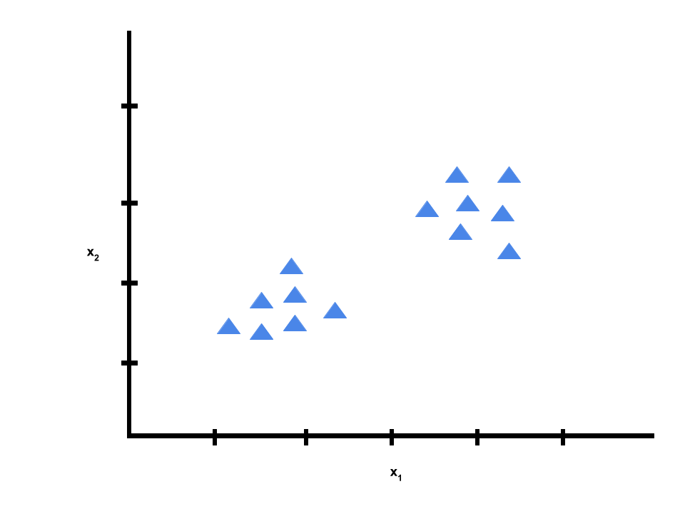
In supervised learning, we have datasets where each example was labeled as either a positive or negative example (e.g. donut or bagel). For each example, we were told explicitly what the “right answer” is.

In unsupervised learning, we are given data that does not have any labels. We’re given a dataset, and our goal is to find some type of structure in the data.

Given the dataset, an unsupervised learning algorithm might decide that the data lives in two different clusters. This is called a clustering algorithm.

Clustering can be used for many applications, such as
>> Organizing large computer clusters to make data centers work more efficiently
>> Identify cohesive groups of friends in social network analysis
>> Group customers into different market segments to automatically and more efficiently sell or market to your different market segments together
>> Perform astronomical data analysis to get interesting and useful theories about how galaxies are formed

K-Means Clustering

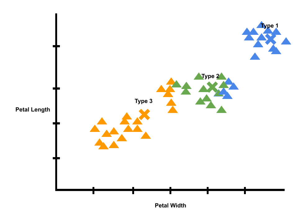
To better understand clustering, let’s look at an example. Let’s say we buy a packet of iris seeds to plant in a garden. After the flowers bloom, it looks like there were several different species of irises mixed up in that one packet. We can use AI to help us analyze the garden.

To construct the model, we need to answer to key questions:
1. What observations can we measure? We could measure color, but all the irises are purple, so that’s not the best way to help tell them apart. But, different irises seem to have different petal lengths and widths.
2. How do we want to represent the world? We will assume that there are k clusters in our data, but we do not know where they are. To help us, we can use the k-means clustering algorithm.

In particular, we want to calculate the mean by adding up all data points in a cluster and dividing by the total number of points.

Let’s start off with k = 3 (i.e., we are looking for three types of irises).

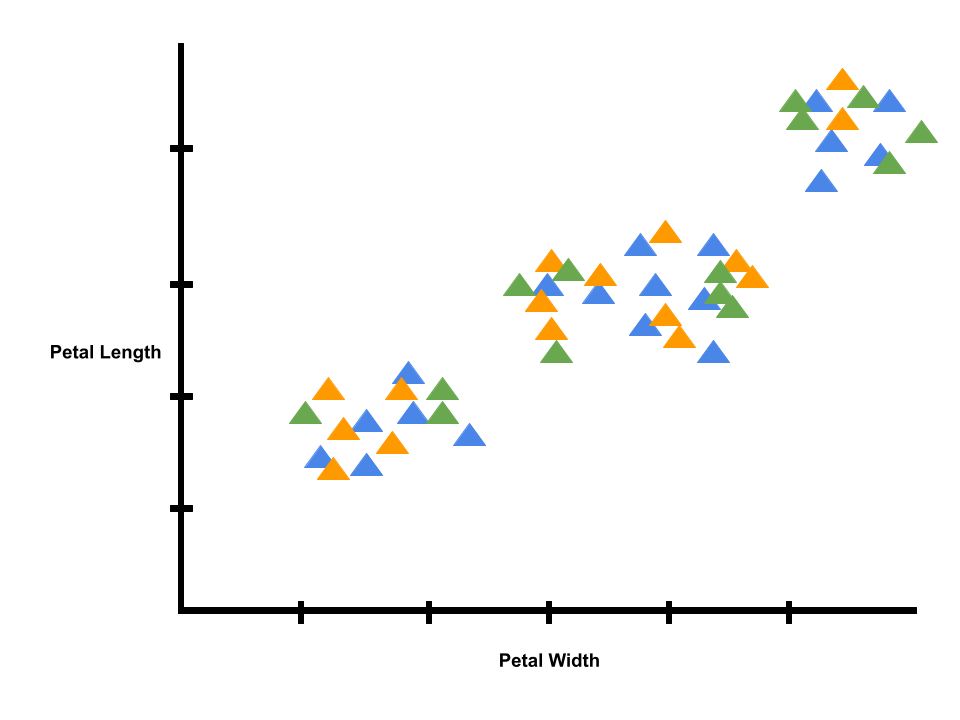
To start, our model doesn’t know anything, so the averages and the predictions are random. Each flower in our dataset is randomly given a label as type 1, type 2, or type 3.

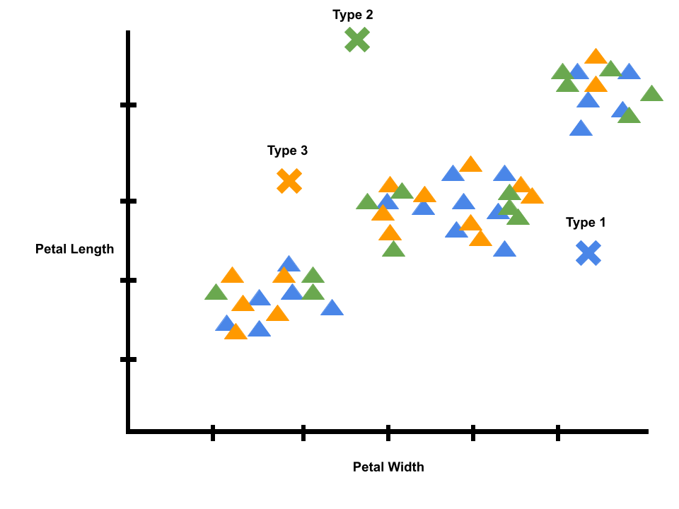
Next, our model tries to correct itself. The average of each cluster of data points should be in the middle. The model corrects itself by calculating new averages, marked by the x’s on the graph. Note that the graph is still pretty noisy. For example, there are many type 2 flowers close to the average of type 3 flowers.

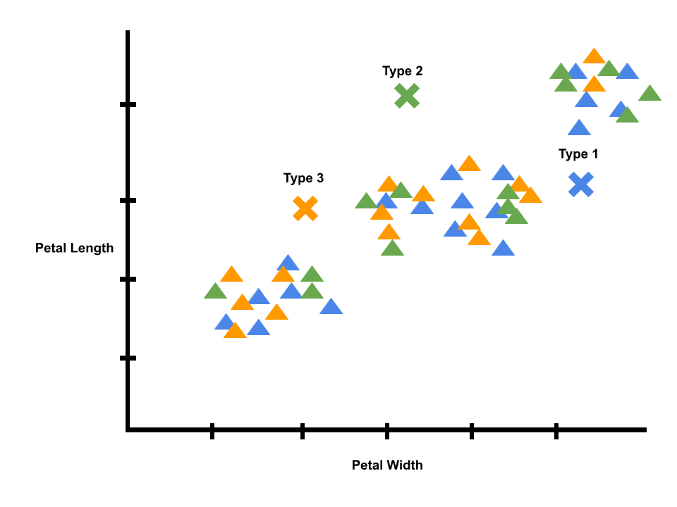
Logically, we know irises of the same species tend to have similar petals. Since we did a correction or learning step, we can repeat the process, starting with a new prediction step. We can predict new labels using the x’s that mark the averages of each label. We will give each datapoint the label of its closest x. Then, we will calculate new averages.

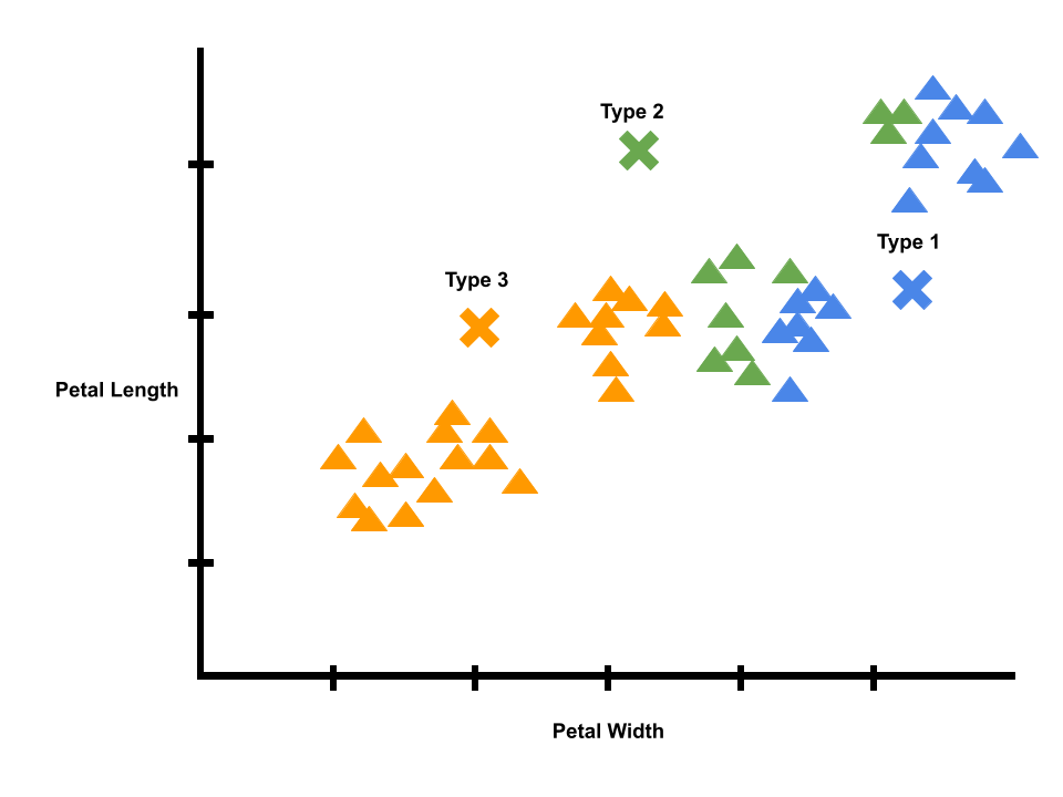
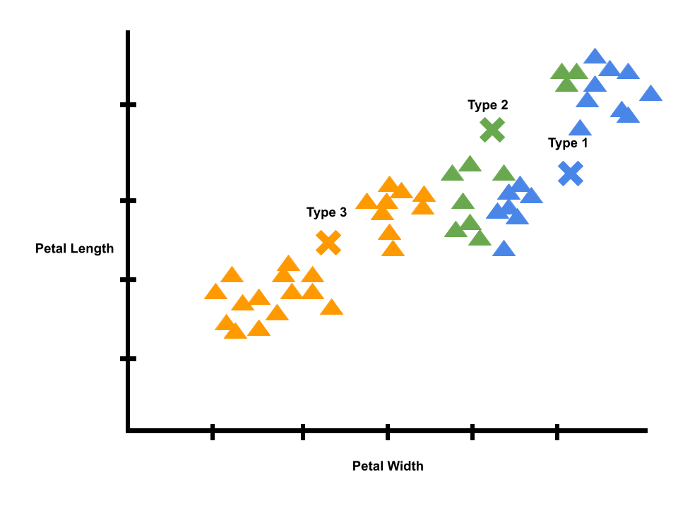
We can repeat the process again. Eventually, the x’s will stop moving, and we will have a model of iris clusters crested with unsupervised learning.

Cocktail Party Algorithm

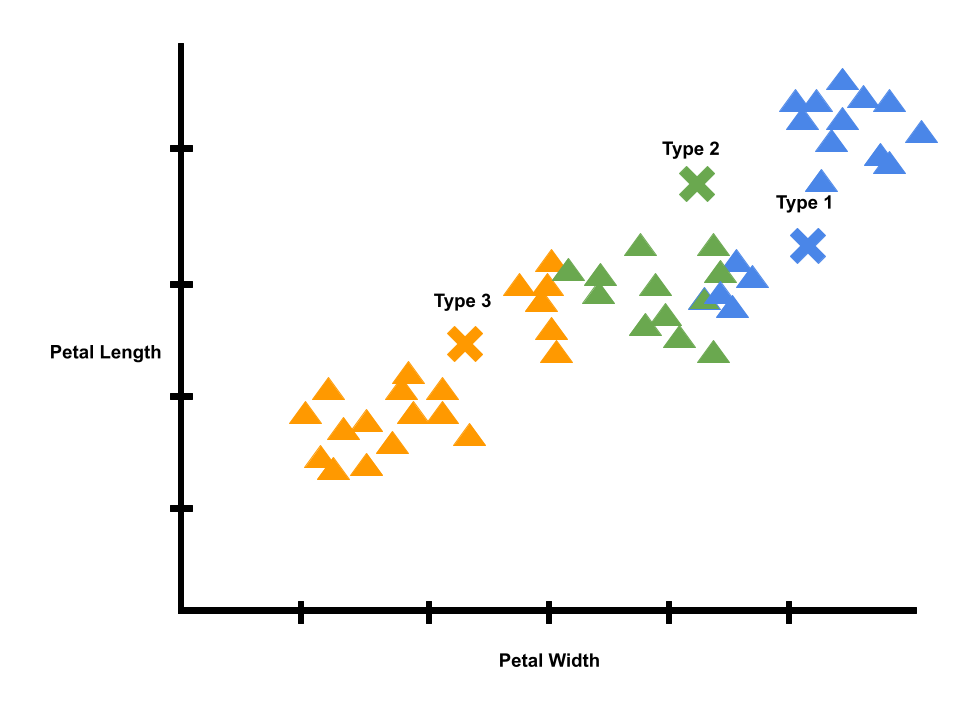
Clustering is just one type of unsupervised learning algorithm. Another unsupervised learning algorithm is known as the cocktail party problem.

Imagine there’s a party room where people are talking to each other, and there are voices overlapping since people are talking at the same time. Suppose there are two people talking at the same time. One of these people is talking to you, and it is hard to hear them. We will put two microphones in the room. Because these microphones are at two different distances from the speakers, each microphone records a different combination of these two speakers' voices.

Suppose in the first microphone recording, we hear someone counting in english and someone counting in spanish at the same time. Speaker 1 is louder in microphone 1 and speaker 2 is louder in microphone 2 because the two microphones are at different positions relative to the two speakers.

We will provide the cocktail party algorithm with these two recordings, and ask the algorithm to find structure in the data. The algorithm will listen to these audio recordings and say that the two audio recordings are being added together to produce the two recordings. Moreover, the cocktail party algorithm will separate the two audio sources that were being added together to form our recordings.

Sources

1. Lecture 1.3 - Unsupervised Learning - Machine Learning by Andrew Ng
2. Unsupervised Learning: Crash Course AI #6

Close Lesson

Reinforcement Learning

Lesson 7

We learn lots of things by trial-and-error. This kind of “learning by doing” to achieve complicated goals is called Reinforcement Learning. Reinforcement Learning is particularly useful for situations where we want to train AIs to have certain skills we don’t fully understand ourselves.

For example, I’m pretty good at walking, but trying to explain the process of walking is kind of difficult. With reinforcement learning, we can train AIs to perform complicated tasks. Unlike other techniques, we only have to tell them at the very end of the task if they succeeded, and then ask them to tell us how they did it.

Here are some real world examples of where RL is useful:
>> Self-driving cars: cars can use computer vision (to see roads, other cars, pedestrians, etc) and route guidance features (e.g. maps, GPS) to learn control braking, acceleration, turning, and more
>> Game bots: We could build an agent to play a game in which we can write down the rules and logic
>> Business Analytics: We could train an agent to buy or sell stocks based on a variety of stock market indicators

If we want an AI to learn to walk, we give them a reward if they’re both standing up and moving forward, and then figure out what steps they took to get to that point. The longer the AI stands up and moves forward, the longer it’s walking, and the more reward it gets. The key to reinforcement learning is just trial-and-error.

For humans, an example of a reward might be a cookie. For an AI system, a reward is a small positive signal that basically tells it “good job” and “do it again!”.

In reinforcement learning, we have an agent that is going to learn. An agent makes predictions or performs actions, e.g., moving a tiny bit forward, or picking the next best move in a game. The agent performs actions based on its current inputs, which we call the state.

In supervised learning, after each action, we would have a training label that tells our AI whether it did the right thing or not. We can’t do that here with reinforcement learning, because we don’t know what the “right thing” actually is until it’s completely done with the task. This difference actually highlights one of the hardest parts of reinforcement learning called credit assignment. It’s hard to know which actions helped us get the reward and which actions slowed down our AI when we don’t pause to think after every action.

The agent ends up interacting with its environment and takes many actions until it gets a reward. Every time the agent succeeds at its task, we can look back on the actions it took and slowly figure out which game states were helpful and which weren’t.

During this reflection, we’re assigning value to those different game states and deciding on a policy for which actions work best.

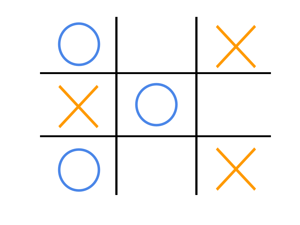
Let’s take a look at an example. Consider the game Tic-Tac-Toe.

The state is the current status of the environment. In the game of tic-tac-toe, the state would be the board and the position of all existing marks. The agent gets to observe the state and then try to choose the optimal action. The agent receives positive rewards for winning and negative rewards for losing/tying. The action is the “move” in which the agent chooses.

Sources

1. Reinforcement Learning: Crash Course AI #9
2. Lecture 9: Reinforcement Learning - High School Machine Learning

Close Lesson

NLP

Lesson 8

Natural Language Processing (NLP) mainly explores two big ideas
1. Natural language understanding: how we get meaning out of combinations of letters. These are AI that filter spam emails, figure out whether a search for “apple” was the fruit or company, and instruct a self-driving car how to get to a friend’s house.
2. Natural language generation: how to generate language from knowledge. These are AI that perform translations, summarize documents, or chat with you.

The key to both problems is understanding the meaning of a word. This is tricky, because words do not have meaning on their own. We assign meaning to symbols. Moreover, in many cases, language can be ambiguous. And, the meaning of a word depends on the context it is used in.

One way to guess which words have similar meaning is to use distributional semantics, i.e., seeing which words appear in the same sentences or not. To make computers understand distributional semantics, we have to use math.

One simple technique is to use count vectors. A count vector is the number of times a word appears in the same article or sentence as other common words. If two words show up in the same sentence, they probably have similar meanings.

Suppose we ask an algorithm to compare the following words using count vectors to guess which of them has similar meaning: car, cat, and felidae. Suppose we download the beginning of the Wikipedia pages for each word to see which other words show up. A lot of the top words are all the same: the, and, of, in. These are all function words or stop words, which help define the structure of language, and help convey precise meaning. “An apple” means any apple, but “the apple” specifies one in particular. Because they change the meaning of another word, they don’t have much meaning by themselves, so we can remove them for now and simplify plurals and conjugations.

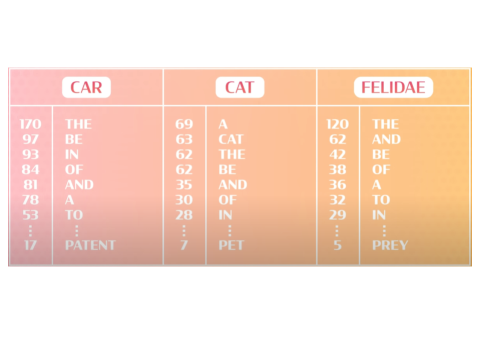
Based on this, it looks like cat and felidae mean almost the same thing, because they both show up with lots of the same words in their Wikipedia articles. Neither of them mean the same thing as car.

One of the problems with count vectors is that we have to store a LOT of data. To compare a bunch of words using counts like this, we’d need a massive list of every word we’ve ever seen in the same sentence, and that’s unmanageable. We’d like to learn a representation for words that captures all the same relationships and similarities as count vectors but is much more compact.

We needed a model that could build internal representations and that could generate predictions. This is where the encoder-decoder model comes in: the encoder tells us what we should think and remember about what we just read and the decoder uses that thought to decide what we want to say or do.

Language Modeling

Let’s create a game of fill in the blank to see what basic pieces we need to train an unsupervised learning model. This is a simple task called language modeling. If I have the sentence “I’m kinda hungry, I think I’d like some chocolate _____ .”, what are the most likely words that can go in that spot? How can we train a model to encode the sentence and decode a guess for the blank?

I can guess the answer might be “cake” or “milk” but probably not something like “potatoes.” The group of words that can fill in that blank is an unsupervised cluster that an AI could use. For this sentence, our encoder might only need to focus on the word chocolate so the decoder has a cluster of “chocolate food words” to pull from to fill in the blank.

Now let’s try a harder example: “Dianna, a friend of mine from San Diego who really loves physics, is having a birthday party next week, so I want to find a present for ____.”

There are two important things to note here
1. The word Dianna appeared 27 words ago
2. Diana happens to use the pronoun “her”

Thus, we want our encoder to build a representation that captures all these pieces of information from the sentence, so the decoder can choose the right word for the blank.

RNNs

Let’s step away from our high level view of language modeling and try to predict the next word in a sentence anyway with a neural network. To do this, our data will be lots of sentences we collect from things like someone speaking or text from books. Then, for each word in every sentence, we’ll play a game of fill-in-the-blank. We’ll train a model to encode up to that blank and then predict the word that should go there. Since we have the whole sentence, we know the correct answer.

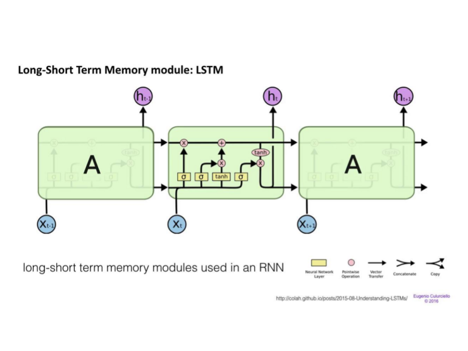
First, we need to define the encoder. We need a model that can read the input sentence. We’ll use a type of neural network called a Recurrent Neural Network or RNN. RNNs have a loop in them that lets them reuse a single hidden layer, which gets updated as the model reads one word at a time. Slowly, the model builds up an understanding of the whole sentence, including which words came first or last, which words are modifying other words, and a whole bunch of other grammatical properties that are linked to meaning.

Now, we can’t just directly put words inside a network. We also don’t have features we can easily measure and give the model either. Unlike images, we can’t even measure pixel values. So, we’re going to ask the model to learn the right representation for a word on its own (note: this is where the unsupervised learning comes in).

We’ll start off by assigning each word a random representation, which in this case is a random list of numbers called a vector. Next, our encoder will take in each of those representations and combine them into a single shared representation for the whole sentence.

At this point, our representation might be gibberish, but in order to train the RNN, we need it to make predictions. For now, we’ll consider a very simple decoder, a single layer network that takes in the sentence representation vector, and then outputs a score for every possible word in our vocabulary.

We can interpret the highest scored word as our model’s prediction. Then, we can use backpropagation to train the RNN, like we’ve done before with neural networks.

By training the model on which word to predict next, the model learn weights for the encoder RNN and the decoder prediction layer. The model changes those random representations we gave every word at the beginning. If two words mean something similar, the model makes their vectors more similar.

This is how we can take in part of a sentence and predict the next word.

Other NLP Tasks

Now, let’s discuss another NLP task. If our model took in English and produced Spanish, we’d have a translation system. Or, our model could read questions and produce answers, like Siri or Alexa try to do.

The representations of words that our model learns for one kind of task might not work for others. For example, if we trained a model based on reading a bunch of cooking recipes, the model might learn that roses are made of icing and placed on cakes. But, the model won’t learn that cake roses are different from real roses.

Acquiring, encoding, and using written or spoken knowledge to help people is a huge and exciting task, because we use language for so many things! Every time you type or talk to a computer, phone or other gadget, NLP is there.

Sources

1. NLP: Crash Course AI #7
2. Understanding LSTM Networks

Close Lesson